
Observation Trip
Had the opportunity to observe at the Los Campanas Observatory in Chile 🇨🇱.

PhD Student at the University of Toronto
LSST DA Data Science Fellow 2025-2027
I am a second year PhD Student in the David A. Dunlap Department of Astronomy & Astrophysics. My current research aims to constrain dark matter and the evolution of our Milky Way through the study of Stellar Streams. My past work studied our polarized radio sky with the CHIME instrument as a part of the Global Magneto-Ionic Mapping Survey.
Had the opportunity to observe at the Los Campanas Observatory in Chile 🇨🇱.
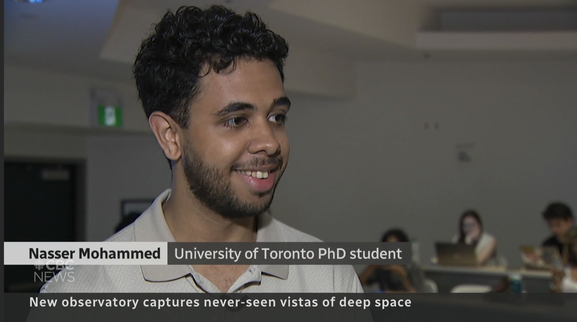
CBC Toronto segment on Dunlap's watch party for the Rubin Observatory's First Look images.
Read more about N. Mohammed & Ordog et al. 2024
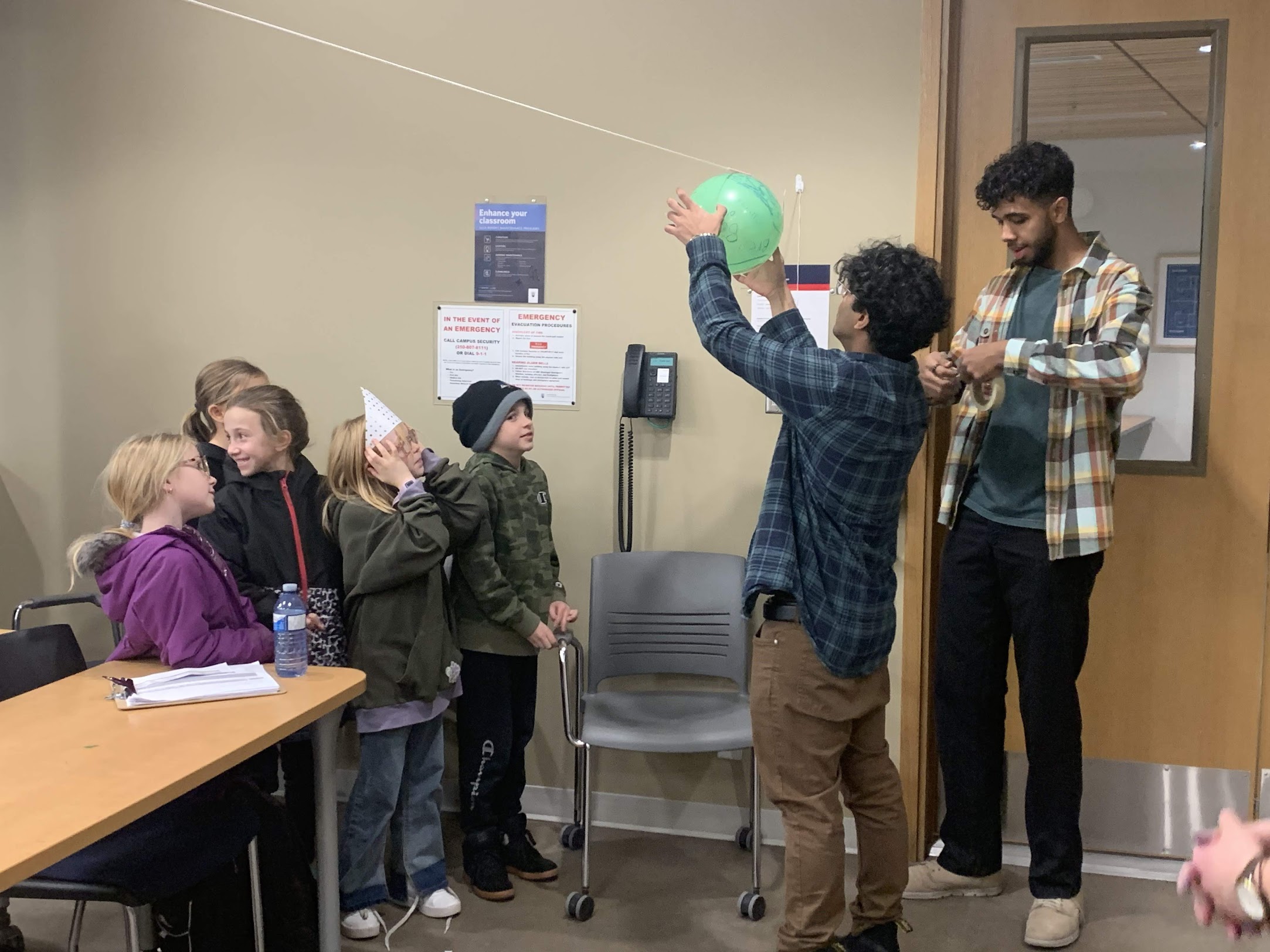
Highlights of recent public outreach efforts.
Milky Way-like galaxies evolved hierarchically, accreting mass through many mergers within a dark matter (DM) halo. Stellar streams are a result of this process; a host galaxy's potential disrupts satellites (dwarf galaxies, globular clusters) leading them to form tidal tails.

Artist depiction of stellar streams in orbit around host galaxy | from S5 Collaboration
Theories of cold and alternative DM disagree on predictions at the sub-galactic scale. Stellar streams offer a powerful means to indirectly constrain the DM substructure within the Milky Way.
However, to do this we need robust membership counts for stellar streams within our Galaxy. There are multiple ways to approach characterizing streams, but in this tutorial you will be walked through using finite mixture models to disentangle stellar streams from surrounding stars.
Mixture models are powerful statistical tools to describe a set of datapoints that come from different distinct populations, even if we can't directly observe which data points belong to which group.
In this tutorial, we will assume that the field of stars we narrow in on can be described by two distinct Gaussian populations: one for the stream, and one for the 'background' (non-stream stars).

Example truncated-Gaussian Mixture Model
We have to fit for the best mixture of models, and to do that we use Bayesian statistics.
$$P(\theta|D) = \frac{\mathcal{L}(D|\theta) \cdot P(\theta)}{P(D)}$$
Where $\mathcal{L}(D|\theta)$ is the likelihood function, $P(\theta)$ is the prior probability, and $P(D)$ is the evidence, with $\theta$ representing our model parameters and $D$ the observed data.
The probability of our model parameters given our observed data is equal to the likelihood of the data given the model parameters multiplied by the prior probability of the model parameters, divided by the probability of the data.
In practice, we can mostly ignore the evidence term ($P(D)$) since it is a constant.
To find the best-fitting parameters, we need to sample from the posterior distribution $P(\theta|D)$. This is where Markov Chain Monte Carlo (MCMC) comes in.
For mixture models, MCMC allows us to simultaneously fit:
The chain explores regions of parameter space with higher posterior probability more frequently, giving us both best-fit values and uncertainty estimates.
I have a tutorial on GitHub that you can use yourself to characterize stellar streams. Run the following terminal command in the directory you'll be working in:
git clone https://github.com/nassmohammed/DESI-DR1_streamTutorial.gitIncluded is:
data/ (small tutorial files), including dotter/, sf3_only_table.csv, and streamfinder_gaiadr3.fits*.py scripts powering the tutorialstreamTutorial.ipynb (the main notebook)env.yml (environment setup)Not included: mwsall-pix-iron.fits (12 GB DESI DR1 stellar catalogue data).
You can download from DESI (see the link in the tutorial) or from your terminal with:
curl -o mwsall-pix-iron.fits https://data.desi.lbl.gov/public/dr1/vac/dr1/mws/iron/v1.0/mwsall-pix-iron.fitsRead the DESI DR1 stellar catalogue overview. The corresponding paper (Kosposov et al. 2025) is here.
If space is a concern, contact ting [dot] li [at] astro [dot] utoronto [dot] ca to get set up on the Eridanus server (for 2025 EXPLORE participants).
Google collab notebook for running on weaker laptops.
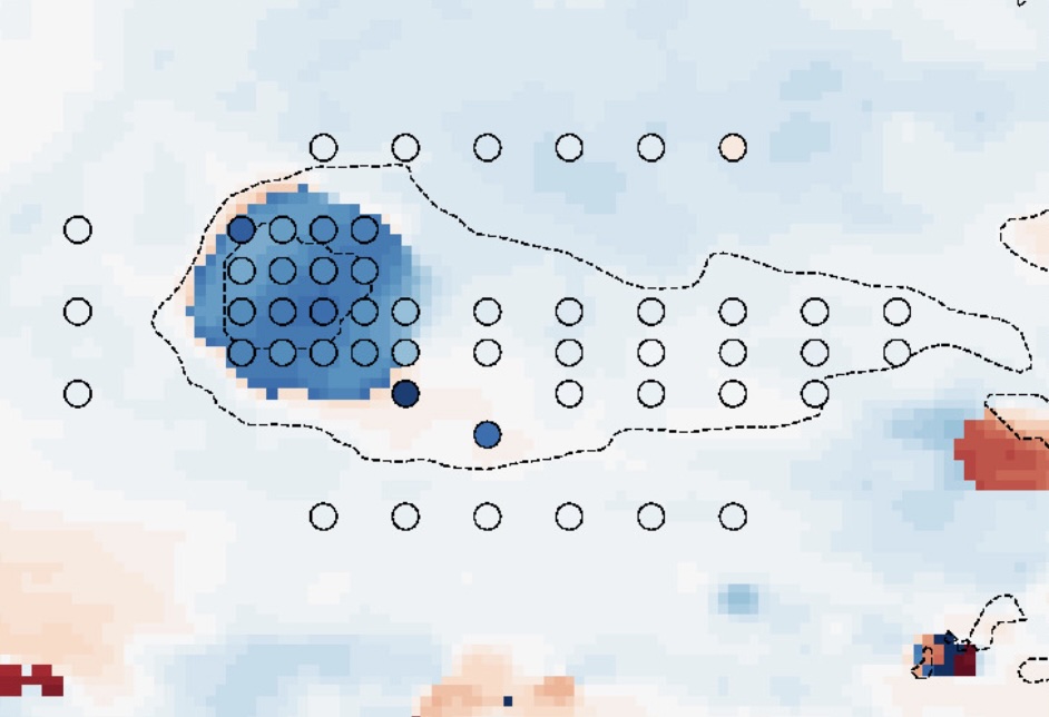
conda env create -f env.ymlbackground = True: show the background stars in the figure for reference.
showStream = True: show STREAMFINDER stars, both those that have survived the cuts (as diamonds) and those cut out (as Xs).
show_sf_only = False: shows STREAMFINDER stars that are NOT IN DESI as hollow diamonds.
show_initial(\optimized\mcmc)_splines = True: shows the respective spline track on top of the figure.
plot_params: a dictionary to change plotting properties without editing the .py file.
Example usage:
plt_kin.plot_params['sf_in_desi']['alpha'] = 0.5
plt_kin.plot_params['sf_in_desi']['zorder'] = 10
plt_kin.plot_params['background']['alpha'] = 0.2
plt_kin.plot_params['background']['s'] = 1A: Don't waste your time. If you have difficulty spotting a stream in the trimmed data, so will the MCMC walkers. Try to adjust your cuts and compare with the location of SF stars.
A: It depends on your device. On Eridanus, 5000 burn-ins with 5000 iterations is about 20 minutes. On Google Colab, about an hour. On an M3 MacBook Pro, about 6 minutes.
A: Diagnostic plots help judge performance: chain plots (watch for hitting an invisible wall or never converging) and corner plots (look for symmetric, well-defined distributions).
@misc{DESI-DR1_streamTutorial,
  author       = {Nasser Mohammed},
  title        = {DESI-DR1\_streamTutorial},
  year         = {2025},
  publisher    = {GitHub},
  journal      = {GitHub repository},
  howpublished = {\url{https://github.com/nassmohammed/DESI-DR1_streamTutorial}},
}Foreman-Mackey, D., Hogg, D. W., Lang, D., & Goodman, J. (2013). emcee: The MCMC Hammer. Publications of the Astronomical Society of the Pacific, 125(925), 306. https://doi.org/10.1086/670067
Ibata, R., et al. (2024). Charting the Galactic Acceleration Field. II. The Astrophysical Journal, 967(1), 89. https://doi.org/10.3847/1538-4357/ad382d
Koposov, S. E., et al. (2025). DESI Data Release 1: Stellar Catalogue. arXiv:2505.14787.
Mateu, C. (2023). galstreams. MNRAS, 520(4), 5225–5258. https://doi.org/10.1093/mnras/stad321


Thanks to the LSST-DA Data Science Fellowship Program, which is funded by LSST-DA, the Brinson Foundation, the WoodNext Foundation, and the Research Corporation for Science Advancement Foundation; participation in this program has benefited this work.
How does football/soccer/futbol (hereafter, simply "football") relate to astrophysics? You may see some novelty stats circular about how player X has scored every game played before sunset, or player Y concedes more fouls when Mars is in retrograde. That's the full (tenuous) extent to which astrophysics and football relate. However, with the recent push to implement data and statistics into football clubs' recruitment, team analysis, and more, the tools that are used to study both astrophysics and football have never been more similar.
Want to dig into the full modelling walkthrough? Read the complete piece on Substack.
