Cookbook on Broadening Function determination using the SVD technique

Important: The BF method provides superior resolution and is basically immune to natural broadening of the spectral lines. Thus, you do not have to remove broadened Balmer lines from A- or F-type spectra if such broadening is present also in the spectrally matched template; such lines carry good information on radial velocity. But the method is EXTREMELY sensitive to the presence of line emissions which are not present in the template. If you have emission lines, you better cut these parts off and splice the velocity binned spectra. The matrix inversion step hates inconsistency and will give you garbage if absorption and emission lines are mixed in the spectra.

This "Cookbook" text is intentionally rather didactic. If you want to go straight into the guts of the method, mostly for the spectroscopic setup used by us at the DDO, read the somewhat more specific description for the DDO programme with comments on IDL routines. All IDL routines mentioned below are also available as BFall_IDL.pro, a combined file of all routines. In IDL, open this file and then compile all routines in one go; this may have to be done several times to re-link routines as they are compiled.

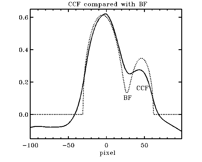Why to use the BF (broadening function) rather than CCF (cross-correlation function)? This picture tells the whole story: The BF is a true linear de-convolution, with the proper baseline at zero and no distortions, while the CCF is a non-linear proxy of the BF showing "peak pulling" or "peak pushing away" effects (due to addition rather than cancellation of common broadening effects and the interaction with the secondary fringes), funny (i.e. wrong) baseline and all sorts of distortions that you want to avoid. But, if you are reading this cookbook, you are probably already convinced ...

And now a disclaimer in the normal friendly spirit of software manuals and books: I assume no responsibility whatsoever for any problems due to my mistakes or your mistakes ...

Iif you do use my routines, I would appreciate mentioning this in your publication. The best references are: Rucinski, S. M., 1992, AJ, 104, 1968 (DDO-7) and Rucinski, S. M., 2002, AJ, 124 1746, or some from the list below (if you find them useful).

This description will be easier to follow if the reader:
[1] ... has access to IDL Version 4 or higher, and ...
[2] ... has read my paper from the conference in Izmir, Turkey in 1998 (17 pages in .ps format).
[3] ...has read a simplified exposition which is shorter than the lengthy paper [2] (8 pages) and is more accessible. Its reference: Rucinski, S.M. 1999, IAU Coll.170, "Precise Stellar Radial Velocities", eds. J.B. Hearnshaw and C.D.Scarfe, ASP Conf.Vol.185, p.82.
You may also want to consult:
[4] - a short note why BF is better than CCF ((the Cancun 2002 conference paper).

As to the IDL versions: A major change in the array multiplication was introduced in the Version 4, so that what is described below applies to Versions 4 and 5. Version 4 accepted array/vector indices in ordinary parentheses (), while Version 5 requires use of the square brackets [] for that purpose. The routines below follow the Version 5 conventions and it is best not to try any earlier version of IDL. IDL is a product of Research Systems Inc. and is protected by copyright and trademark conventions.

A self-contained Windows application has been written by Bob Nelson. If you want to avoid IDL, you can copy Bob's ready for use program from BobNelson.zip. I still suggest that you read the explanations below as the program of Bob assumes that the reader knows what he/she is doing...

1. Reading in the FITS spectra

Read in your spectra into IDL. Reading in ascii files is part of what is described in IDL manuals, so I skip that. Routines from the Astro-IDL library are very useful for FITS spectra (and for ascii tabular data in columns). Pay special attention to the compatibility of the IDL versions. Since the FITS standard is not very strict, you may want to try various FITS readers given there. The routine readfits.pro usually works well, although it is known to give problems when IDL-4 and IDL-5 versions are mixed up (it uses several other routines from the IDL-astro package, all must be compatible).

If the standard spectrum will be called ss and the program spectra will be sp1, sp2, ..., read them in as follows (remember that before use, each routine must be compiled with: .run routine_name - without the .pro extension):

 
ss=readfits('file-std.fits',hs) 
sp1=readfits('file-p1.fits',hp1) 
sp2=readfits('file-p2.fits',hp2)

Although the headers do not have to be read with readfits.pro, it is easier to use the header data contained in simple string arrays such as hs, hp1, hp2 in restoration of the wavelength scale for each spectrum. In the FITS files, the relevant data are usually under: CRVAL1 and CDELT1 (starting wavelength and increment). Write down these numbers for each spectrum (they will be different because of the heliocentric corrections already applied to the wavelengths) and then create the wavelength vectors ws, wp1, wp2.

Say, for CRVAL1=5185 and CDELT1=0.0215: ws=5185.0+0.0215*findgen(1024)
Here 1024 is an example of the actual length in pixels. Usually, it will be the same as for ss, sp1, sp2 etc., but the exactly same length is not crucial because the spectra will be re-sampled to log(wave) scale anyway. In fact, typical IRAF reductions with removal of blemishes at ends of the spectra may have resulted in a smaller number than 512, 1024, 2048, etc, so check the length of ss, sp1, sp2 using the statement

Help

in IDL and make the corresponding vectors, sp, w of the same length.

At the end of this step, you should have the data and wavelength vectors for each spectrum. The headers will not be needed, but you can keep them.

Important: Usually, normalized spectra are used in the process. This way one avoids any influence of the sloping continuum. However, for a proper handling of the ends (where a jump from unity to zero would occur), it is important to convert spectra to a form in which the absorption lines are represented by positive spikes. Then the ends are usually close to zero, but the content is not changed in terms of the usefullnes for the de-convolution.

ss=1.-ss
sp1=1.-sp1
sp2=1.-sp2
etc

2. Re-sampling to equal velocity (log lambda) steps

Now we will create one vector of wavelengths which will serve all spectra and will be in equal increments of log lambda.

The pixel spacing determines the velocity spacing, delV. If you take the high wavelength end of the spectrum and divide CDELT1 by the wavelength at this point, you will have an optimal spacing. However, any round number will be fine as long as you sample at a frequency close to or higher than the original sampling (this will preserve the information content).

Say, you decide on velocity resolution delV=12 km/s. Then you will create one wavelength vector for all spectra, w1:

 
r = 12.0/2.997924d5
w1 = 5187.0 * (1.d0+r)^dindgen(1024)

r is the inverse of the spectroscopic resolution R. Note that we started at 5187. This was selected to be a safe, same start for all spectra. Some of them could have the first pixel at 5185.5 or at 5186.2 (due to heliocentric corrections), so one must check all spectra where they actually begin and select a good common start. This is an important step because you are setting the relative velocity scale for all spectra. The resulting BF will be in relative velocity scale, program star minus standard (template) star. It may be prudent to check how far the spectra go, so in this example, check if the last element (in our case: w1[1023]) is safely within the ranges of ws, wp1, wp2.

The re-sampling is through a simple linear interpolation:

 
ssr=interpol(ss,ws,w1)
sp1r=interpol(sp1,wp1,w1)
sp2r=interpol(sp2,wp2,w1)

The size of the vector w1 and of the re-sampled spectra is called n in the text. Recall that it is pretty arbitrary and does not have to be 1024 or anything like that, but should be close to (or slightly larger than) the number of pixels in the original spectra. For the BF determination as described below in Sec.4, the number of pixels should be even.

3. Cross-correlation function (CCF)

If you like, you can cross-correlate your spectra to have some idea what is there. Suppose your span in velocities is 2400 km/s sampled at 12 km/s. Then, for 201 pixels centred at zero, with 100 elements each way, use:

 
lag = findgen(201)-100 ; lag vector
ccf1 = c_correlate(ssr,sp1r,lag) ; correlation ssr with sp1r
ccf2 = c_correlate(ssr,sp2r,lag) ; correlation ssr with sp2r
vel = lag*12.
plot,vel,ccf1

Note that the sense of the CCF is: How much to shift the template to fit the program spectrum, not the reverse...

For many applications, such as single-object radial-velocity determinations, CCF's are totally adequate and you do not have to go into the pain of the broadening function derivation (no, it is not a pain, actually a lot of fun...).

4. Broadening functions, part I: Analysis of the standard spectrum

If you have one standard spectrum, you will have to go through this step only once. It is prudent to use a few standard spectra with slightly different spectral types. The S/N should be as high as possible, but if it is not, the SVD technique will take care of the noise and will attempt to remove it by telling you this through the plot of the vector of Singular Values, ww, as below. The determination will be poorer, of course.

The design matrix, des is formed using a simple procedure map4.pro utilizing many internal loops. Typical use is:
des = map4(ssr,201)

The span has been selected again 201 pixels, although it can be any other odd number. A few cautionary notes are in order here: (1) Running of map4 may take several minutes even on relatively fast computers, mostly because of the very inefficient loop structure within the routine. (2) The resulting BF will be centered on the zero relative velocity, so that the routine is not very well suited for handling very large velocity differences which arise when dealing with PopII objects or red-shifted galaxies. In such situations, one must either set up a wide window and then accept that the BF will be defined at one end of it or one must make slightly longer velocity-rebinned spectra and just shift them relative to the template by a known and fixed number of pixels. (3) Currently, because of the integer index limitation of the IDL, the routine can only handle spectra which are shorter than 32,000 pixels. This limitation is becoming more important with new echelle spectrographs producing very long spectra. The routine is prohibitively inefficient when the integer indices are replaced by long integers.

The map4.pro routine is as follows:

 
function map4,x,m
; version for IDL 4.0 and higher (SMR Feb.15'97)
; shifts vectors x vertically within m
; for broadening functions
 t=0 
 n=n_elements(x)
 if n gt 32000 then begin
 print,'n - too large' & goto,E
 end
 if (m mod 2) ne 1 then begin
 print,'m - must be odd' & goto,E 
 end
 if (n mod 2) ne 0 then begin
 print,'n must be even' & goto,E
 end
 t = fltarr(m) # fltarr(n-m+1) ; t(m,n-m)=
 ; t(small,large-small) dimensions
 for j=0,m-1 do $
 for i=m/2,n-m/2-1 do t(j,i-m/2)=x(i-j+m/2)
E: return,t
end

The SVD step will create 3 arrays, ww, u, v:

svdc,des,ww,u,v,/double 

Again, this step may be slow on some computers. It is now essential to plot ww. It is stored as a vector, but these are actually diagonal elements of a square array. Because of the very large range in size of the elements of ww (most of information about the BF is in the first few elements), the best is to use the lin-log plot:

plot_io,ww 

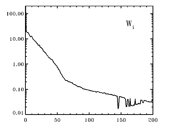Consult Fig.8 in the paper (shown here). Your plot will look a bit similar. Note the bends/kinks in the plot. For the case shown in Fig.8, you would definitely want to write down that the SVD technique encountered numerical noise at and beyond the index of ww (=W_i) of about i=140. You may also suspect, that the kink at about i=65 indicates that (1) the featureless continuum starts to be represented by these singular values and/or (2) that noise starts to show up about there. Since the cause (2) depends on the S/N of the standard spectrum, you can test that.

5. Broadening functions, part II: Processing of the program spectra

For each program spectrum, you must form its slightly truncated version (bottom page 7 in the paper):
sp1rt=sp1r[201/2:1024-201/2-1]
sp2rt=sp2r[201/2:1024-201/2-1]

I entered the specific numbers for illustration, but you can use a small routine to process these spectra, like the following routine trunc.pro:

function trunc,spec,m,n
; must be: m-odd, n-even
 return,spec[m/2:n-m/2-1]
end

Which can be used as:

 
sp1rt=trunc(sp1r,201,1024) 
sp2rt=trunc(sp2r,201,1024) 

For each program spectrum, you will form an array of the BF solutions, say, bb. This can be achieved using the following subroutine broadfunct.pro:

pro broadfunct,sp,w,u,v,m,bb
 bb=fltarr(m,m)
 for i=0,m-1 do begin
 wb=fltarr(m)
 wb[0:i]=w[0:i]
 bb[*,i]=svsol(u,wb,v,sp,/double)
 end
return
end

Using this routine, the individual broadening functions can be recovered using:

 
braodfunct,sp1rt,ww,u,v,201,bb1
braodfunct,sp2rt,ww,u,v,201,bb2

6. Broadening functions, part III: What to do with the broadening function arrays (Route #1)?

The consecutively better estimates of the broadening functions are the consecutive rows of the bb arrays. You must select the best among them, i.e. giving the most structure, yet without much of error sneaking in. The last row (in our case bb1[*,200]) gives the full resolution solution. Note that the elements of this solution are un-correlated with each point simply being treated as an unknown. There is no smoothing and no information on continuity for this last row. But the rows before the last do show inter-correlation between the elements because some basis functions of the de-convolution are missing. A description of an alternative approach is given in Sec.7 below.

So, how far to go? By now we have some idea that, in the specific case as in the paper, there is no point of using any of the bb1, bb2 beyond the row [*,140]; even [*,65] may be suspicious. Now you can plot these solutions using the relative velocity vector:
vel=12.*(findgen(201)-100)
(of course delV=12. may be different in your case):
plot,vel,bb[*,65]

This will give you a decent result, but this is not the end of the story. Index 65 is probably still too high. The numerical noise in the SVD decomposition has been taken care of, but there is still the genuine problem of the linear dependencies (featureless continuum mapped into featureless continuum). At this point one must ask: "How many singular values ww[i] in the BF do I need to reproduce my spectrum?". Usually, the answer is: "Far fewer than one would imagine". The proper way is through analysis of the std deviation of the fit. One should stop at the point where the fit stops improving. If you use too many ww[i], you just reproduce the noise in the spectrum, not its real shape.

One can use the following routine to obtain the vector sig representing the error of fit:

 
function sig,des,bb,sp
 m = n_elements(bb[0,*]) ; size of vector
 sig=fltarr(m) ; temporary array
 pred = des ## transpose(bb) ; predicted spectrum
 for i=0,m-1 do sig[i]=sqrt(total((pred[i,*]-sp)^2)/m)
return,sig
end

You would run this function as:

 
sig1 = sig(des,bb1,sp1rt)
sig2 = sig(des,bb1,sp2rt)

Now check where the error stabilizes. It is important to plot the range from zero, not over the observed range in y-coordinate, as follows:
plot,sig1,yran=[0,1.1*max(sig1)]

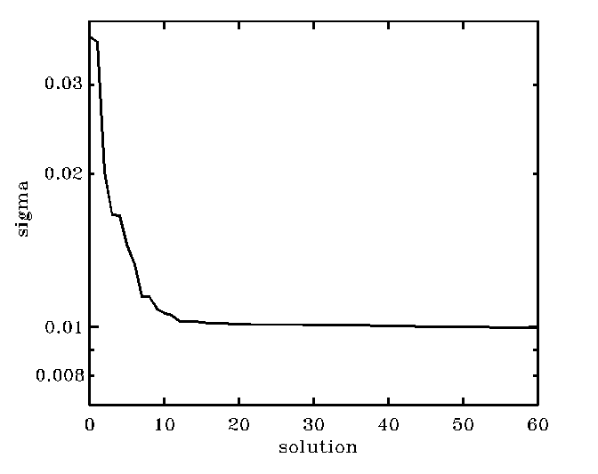In the case in Fig.11 in the paper (shown here), the plot suggests that index as low as i=15 is sufficiently high and that bb[*,15] is a good solution. This way we would discard some 185 solutions from among 201 solutions which contain just progressively more noise. If you want to feel better by seeing some wiggly noise to creep into your results, use bb[*,20], but do not go much further than that! A bit of feeling for art helps here.

The result of the process is a broadening function, say,
bbb=reform(bb[*,20])
(the IDL instruction reform simplifies the vector to strictly 1-D) which should be plotted versus the velocity vector:
plot,vel,bbb
The function can be used for modeling of the star with spots, for determination of Vsini or for measurements of radial velocities of components in a binary system. But this is astrophysics where you know more about the particular problem so I stop making suggestions here ...

The approach described above, through rejection of - what we presume - insignificant contributions to BF, will be called here Route#1. It carries a certain danger for radial-velocity determinations in that the BF's may be slightly skewed (some basis vectors are rejected). For that reason we currently prefer an alterantive approach, as described below.

7. An alternative approach (Route#2)

As we said at the beginning of Sec.6 above, no information on continuity of the BF exists in the last row of the solutions (in our case bb[*,200]). All points of the solution are independent of each other. But one can introduce such correlation between the elements by choosing a particular solution, such as say,
bbb=reform(bb[*,20])
This is because many basis functions are then removed and the total independence of the elements of the solution is lost. True, such a solution is the best you can get to reproduce the observed spectrum, down to the mean deviation sig. However, especially for radial velocity applications, when one is ready to accept some random noise in the BF definition, but would rather prefer not to have any systematic distortions, you may try a different way...

One can do the following: Select the last row in the broadening-function array (the full resolution one) and smooth it with a Gaussian. This way you will be using the powerful property of the full solution that the elements are totally un-correlated. By smoothing, you remove mostly the un-correlated, small-scale noise and obtain a better solution. This in fact appears to me a better approach than removal of many (mathematically seemingly irrelevant) singular values as their absence may introduce some unwanted systematic effects. Besides, the instrumental setup usually leads to some local averaging in the sense that the projection of the spectrograph slit image on the CCD is usually selected to be of the order of 2-3 pixels wide. Any noise at finer scales must be then caused by the matrix inversion process.

How to do that? Define a smoothing Gaussian with the following function:

function gs_smooth,n,sigma
;
; prepares a n-element vector of total area=1 and Gaussian shape
; given by sigma, shifted to the origin [bbb.....bbb]
; for Gaussian filter using new=cnv(old,gs_smooth)
;
; when a given FWHM needed, use relation: FWHM = 2.354 sigma
; or: sigma = 0.4248 FWHM
 b = findgen(n)
 c = b
 c = ((b - b(n/2))/sigma)^2/2
 b(*) = 0.
 d = where(c le 30.) 
 b(d) = exp(-c(d))
 b = shift(b, -n/2)
return, b/total(b)
end

so that you first prepare the smoothing Gaussian (here for sigma=3.0) and then use it for smoothing:

gs30=gs_smooth(201,3.0)
bb30=cnv(reform(bb[*,200]),gs30)

The convolution can be accomplished using the following compact IDL function cnv.pro:

function cnv,a,b
; [SMR: 10 Oct 1992]
; general convolution of two vectors or arrays with same dimensions;
; vector or array b must be symmetric at ends: [bbb........bbb]
; and normalized to integral = 1 (for Gaussians, use gs_smooth for 1-D
; and gs2_smooth for 2-D
;
; usage: new_vector=cnv(vector,smoothing_vector)
; 
 return,float(fft(fft(a,-1)*fft(b,-1),+1)*float(n_elements(a)))
end

(by the way: I prefer this one over the convol.pro of IDL, although it may fail at the ends if the functions do not converge to zero there; the inverted spectra with absorption lines as positive spikes usually do).

Which solution is better? Route#1 with high-order singular values removed (as in Secs.5 and 6) or Route#2 which uses the full resolution, with noise removed by smoothing (as above)? Frankly, I don't know. I hope to find out this one day... The former is more elegant mathematically, the latter really guarantees that the result will have no hidden distortions due to missing basis functions. Both are perfectly legitimate approaches.

8. Fitting Gaussians for binary stars

This is a specialized application: Having the broadening function bbb defined over the velocity span vel, one can determine the binary radial velocities using Gaussian fits. Note that least-squares Gaussian fits are usually unstable and that fixing of the widths of the components usually helps. I give four IDL routines to accomplish the fits.

---

Slavek Rucinski, updated March 2005
Please let me know if something is unclear or wrong by e-mail: rucinski@astro.utoronto.ca